Another Word For It Patrick Durusau on Topic Maps and Semantic Diversity

August 3, 2016

Interactive 3D Clusters of all 721 Pokémon Using Spark and Plotly

Filed under: Clustering,Plotly,Spark,Visualization — Patrick Durusau @ 10:26 am

Interactive 3D Clusters of all 721 Pokémon Using Spark and Plotly by Max Woolf.

721-pokemon-460

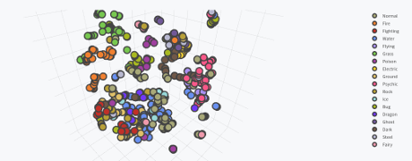
My screen capture falls far short of doing justice to the 3D image, not to mention it isn’t interactive. See Max’s post if you really want to appreciate it.

From the post:

There has been a lot of talk lately about Pokémon due to the runaway success of Pokémon GO (I myself am Trainer Level 18 and on Team Valor). Players revel in the nostalgia of 1996 by now having the ability catching the original 151 Pokémon in real life.

However, while players most-fondly remember the first generation, Pokémon is currently on its sixth generation, with the seventh generation beginning later this year with Pokémon Sun and Moon. As of now, there are 721 total Pokémon in the Pokédex, from Bulbasaur to Volcanion, not counting alternate Forms of several Pokémon such as Mega Evolutions.

In the meantime, I’ve seen a few interesting data visualizations which capitalize on the frenzy. A highly-upvoted post on the Reddit subreddit /r/dataisbeautiful by /u/nvvknvvk charts the Height vs. Weight of the original 151 Pokémon. Anh Le of Duke University posted a cluster analysis of the original 151 Pokémon using principal component analysis (PCA), by compressing the 6 primary Pokémon stats into 2 dimensions.

However, those visualizations think too small, and only on a small subset of Pokémon. Why not capture every single aspect of every Pokémon and violently crush that data into three dimensions?

If you need encouragement to explore the recent release of Spark 2.0, Max’s post that in abundance!

Caveat: Pokémon is popular outside of geek/IT circles. Familiarity with Pokémon may result in social interaction with others and/or interest in Pokémon. You have been warned.

February 24, 2016

Open-Source Sequence Clustering Methods Improve the State Of the Art

Open-Source Sequence Clustering Methods Improve the State Of the Art by Evguenia Kopylova et al.

Abstract:

Sequence clustering is a common early step in amplicon-based microbial community analysis, when raw sequencing reads are clustered into operational taxonomic units (OTUs) to reduce the run time of subsequent analysis steps. Here, we evaluated the performance of recently released state-of-the-art open-source clustering software products, namely, OTUCLUST, Swarm, SUMACLUST, and SortMeRNA, against current principal options (UCLUST and USEARCH) in QIIME, hierarchical clustering methods in mothur, and USEARCH’s most recent clustering algorithm, UPARSE. All the latest open-source tools showed promising results, reporting up to 60% fewer spurious OTUs than UCLUST, indicating that the underlying clustering algorithm can vastly reduce the number of these derived OTUs. Furthermore, we observed that stringent quality filtering, such as is done in UPARSE, can cause a significant underestimation of species abundance and diversity, leading to incorrect biological results. Swarm, SUMACLUST, and SortMeRNA have been included in the QIIME 1.9.0 release.

IMPORTANCE Massive collections of next-generation sequencing data call for fast, accurate, and easily accessible bioinformatics algorithms to perform sequence clustering. A comprehensive benchmark is presented, including open-source tools and the popular USEARCH suite. Simulated, mock, and environmental communities were used to analyze sensitivity, selectivity, species diversity (alpha and beta), and taxonomic composition. The results demonstrate that recent clustering algorithms can significantly improve accuracy and preserve estimated diversity without the application of aggressive filtering. Moreover, these tools are all open source, apply multiple levels of multithreading, and scale to the demands of modern next-generation sequencing data, which is essential for the analysis of massive multidisciplinary studies such as the Earth Microbiome Project (EMP) (J. A. Gilbert, J. K. Jansson, and R. Knight, BMC Biol 12:69, 2014, http://dx.doi.org/10.1186/s12915-014-0069-1).

Bioinformatics has specialized clustering issues but improvements in clustering algorithms are likely to have benefits for others.

Not to mention garage gene hackers, who may benefit more directly.

February 17, 2015

Clustering by Descending to the Nearest Neighbor in the Delaunay Graph Space

Filed under: Clustering,Graphs — Patrick Durusau @ 5:37 pm

Clustering by Descending to the Nearest Neighbor in the Delaunay Graph Space by Teng Qiu and Yongjie Li.

Abstract:

In our previous works, we proposed a physically-inspired rule to organize the data points into an in-tree (IT) structure, in which some undesired edges are allowed to occur. By removing those undesired or redundant edges, this IT structure is divided into several separate parts, each representing one cluster. In this work, we seek to prevent the undesired edges from arising at the source. Before using the physically-inspired rule, data points are at first organized into a proximity graph which restricts each point to select the optimal directed neighbor just among its neighbors. Consequently, separated in-trees or clusters automatically arise, without redundant edges requiring to be removed.

The latest in a series of papers exploring clustering issues. The author’s concede the method demonstrated here isn’t important but represents another step in their exploration.

It isn’t often that I see anything other than final and “defend to the death” results. Preliminary and non-successful results being published will increase the bulk of scientific material to be searched but it will also leave a more accurate record of the scientific process.

Enjoy!

January 4, 2015

When Similarity Breaks Down

Filed under: Clustering,Similarity — Patrick Durusau @ 7:21 pm

From the description:

Clustering data is a fundamental technique in data mining and machine learning. The basic problem can be specified as follows: “Given a set of data, partition the data into a set of groups so that each member of a given group is as similar as possible to the other members of that group and as dissimilar as possible to members of other groups”. In this talk I will try to unpack some of the complexities inherent in this seemingly straightforward description. Specifically, I will discuss some of the issues involved in measuring similarity and try to provide some intuitions into the decisions that need to be made when using such metrics to cluster data.

iPython notebook, useful because the slides don’t show up well in the video. (Be aware the github link is broken.)

Nothing new but Bart does a good job of pointing out that similarity breaks down with high dimensionality. The more dimensions that you are representing in Euclidian space, the less distance there will be along some of those dimensions.

At our evening meal today, I was telling my wife about how similarity breaks down under high dimensionality and she recalled a story about how an autistic child was able to distinguish dogs from cats.

The child had struggled to make the distinction for a number of years and then one day succeeded and was able to distinguish dogs from cats.

Think of distinguishing dogs and cats as a high dimensionality problem:

Dimension Cat Dog
4 legs Y Y
2 eyes Y Y
2 ears Y Y
fur Y Y
tail Y Y
color Y Y
mammals Y Y
pet Y Y
jumps Y Y
runs Y Y
plays Y Y
toys Y Y

There’s twelve that a child would notice. It could go a lot higher with more technical information.

The high number of dimensions won’t help an autistic child distinguish dogs from cats. Not likely to help a machine algorithm either.

When the child did learn how to distinguish dogs from cats, they were asked what had helped them tell the difference between dogs and cats?

The child responded that they looked only at the end of the nose of any animal presented as a dog or a cat to tell the difference. In machine learning lingo, they reduced all the dimensions above and many others to a single one. That one dimension was enough to enable them to reliably tell dogs from cats.

Like you, I had to go find images to see if this was possible:

220px-Kittyply_edit1

220px-Border_Collie_liver_portrait

Do you see it?

The shape of a cat’s nose, just the end of it, is a distinct T shape.

The shape of a dog’s nose, just the end of it, is round.

Every time. T versus round.

I can’t think of a better illustration of breaking down of similarity in high dimensions or of the power of dimensional reduction.

A topic for another day but it also makes me wonder about dynamically choosing dimensions along which to identify subjects.

November 29, 2014

VSEARCH

Filed under: Bioinformatics,Clustering,Merging,Topic Maps — Patrick Durusau @ 4:15 pm

VSEARCH: Open and free 64-bit multithreaded tool for processing metagenomic sequences, including searching, clustering, chimera detection, dereplication, sorting, masking and shuffling

From the webpage:

The aim of this project is to create an alternative to the USEARCH tool developed by Robert C. Edgar (2010). The new tool should:

  • have open source code with an appropriate open source license
  • be free of charge, gratis
  • have a 64-bit design that handles very large databases and much more than 4GB of memory
  • be as accurate or more accurate than usearch
  • be as fast or faster than usearch

We have implemented a tool called VSEARCH which supports searching, clustering, chimera detection, dereplication, sorting and masking (commands --usearch_global, --cluster_smallmem, --cluster_fast, --uchime_ref, --uchime_denovo, --derep_fulllength, --sortbysize, --sortbylength and --maskfasta, as well as almost all their options).

VSEARCH stands for vectorized search, as the tool takes advantage of parallelism in the form of SIMD vectorization as well as multiple threads to perform accurate alignments at high speed. VSEARCH uses an optimal global aligner (full dynamic programming Needleman-Wunsch), in contrast to USEARCH which by default uses a heuristic seed and extend aligner. This results in more accurate alignments and overall improved sensitivity (recall) with VSEARCH, especially for alignments with gaps.

The same option names as in USEARCH version 7 has been used in order to make VSEARCH an almost drop-in replacement.

The reconciliation of characteristics that are different is the only way that merging in topic maps varies from the clustering found in bioinformatics programs like VSEARCH. The results are a cluster of items deemed “similar” on some basis and with topic maps, subject to further processing.

Scaling isn’t easy in bioinformatics but it hasn’t been found daunting either.

There is much to be learned from projects such as VSEARCH to inform the processing of topic maps.

I first saw this in a tweet by Torbjørn Rognes.

November 11, 2014

Massively Parallel Clustering: Overview

Filed under: Clustering,Hadoop,MapReduce — Patrick Durusau @ 3:35 pm

Massively Parallel Clustering: Overview by Grigory Yaroslavtsev.

From the post:

Clustering is one of the main vechicles of machine learning and data analysis.
In this post I will describe how to make three very popular sequential clustering algorithms (k-means, single-linkage clustering and correlation clustering) work for big data. The first two algorithms can be used for clustering a collection of feature vectors in \(d\)-dimensional Euclidean space (like the two-dimensional set of points on the picture below, while they also work for high-dimensional data). The last one can be used for arbitrary objects as long as for any pair of them one can define some measure of similarity.

mapreduce clustering

Besides optimizing different objective functions these algorithms also give qualitatively different types of clusterings.
K-means produces a set of exactly k clusters. Single-linkage clustering gives a hierarchical partitioning of the data, which one can zoom into at different levels and get any desired number of clusters.
Finally, in correlation clustering the number of clusters is not known in advance and is chosen by the algorithm itself in order to optimize a certain objective function.

All algorithms described in this post use the model for massively parallel computation that I described before.

I thought you might be interested in parallel clustering algorithms after the post on OSM-France. Don’t skip model for massively parallel computation. It and the discussion that follows is rich in resources on parallel clustering. Lots of links.

I take heart from the line:

The last one [Correlation Clustering] can be used for arbitrary objects as long as for any pair of them one can define some measure of similarity.

The words “some measure of similarity” should be taken as a warning the any particular “measure of similarity” should be examined closely and tested against the data so processed. It could be that the “measure of similarity” produces a desired result on a particular data set. You won’t know until you look.

I/O Problem @ OpenStreetMap France

Filed under: Clustering,Mapping,Maps,Topic Maps — Patrick Durusau @ 2:54 pm

Benefit of data clustering for osm2pgsql/mapnik rending by Christian Quest.

The main server for OpenStreetMap France had an I/O problem:

OSM-FR

See Christian’s post for the details but the essence of the solution was to cluster geographic data on the basis of its location. To reduce the amount of I/O. Not unlike randomly seeking topics with similar characteristics.

How much did clustering reduce the I/O?

OSM-FR stats

Nearly 100% I/O was reduced to 15% I/O. 85% improvement.

An 85% improvement in I/O doesn’t look bad on a weekly/monthly activity report!

Now imagine clustering topics for dynamic merging and presentation to a user. Among other things, you can have an “auditing” view that shows all the topics that will merge to form a single topic in a presentation view.

Or a “pay-per-view” view that uses a different cluster to reveal more information for paying customers.

All while retaining the capacity to produce a serialized static file as an information product.

August 17, 2014

AverageExplorer:…

Filed under: Clustering,Image Recognition,Indexing,Users — Patrick Durusau @ 4:22 pm

AverageExplorer: Interactive Exploration and Alignment of Visual Data Collections, Jun-Yan Zhu, Yong Jae Lee, and Alexei Efros.

Abstract:

This paper proposes an interactive framework that allows a user to rapidly explore and visualize a large image collection using the medium of average images. Average images have been gaining popularity as means of artistic expression and data visualization, but the creation of compelling examples is a surprisingly laborious and manual process. Our interactive, real-time system provides a way to summarize large amounts of visual data by weighted average(s) of an image collection, with the weights reflecting user-indicated importance. The aim is to capture not just the mean of the distribution, but a set of modes discovered via interactive exploration. We pose this exploration in terms of a user interactively “editing” the average image using various types of strokes, brushes and warps, similar to a normal image editor, with each user interaction providing a new constraint to update the average. New weighted averages can be spawned and edited either individually or jointly. Together, these tools allow the user to simultaneously perform two fundamental operations on visual data: user-guided clustering and user-guided alignment, within the same framework. We show that our system is useful for various computer vision and graphics applications.

Applying averaging to images, particularly in an interactive context with users, seems like a very suitable strategy.

What would it look like to have interactive merging of proxies based on data ranges controlled by the user?

August 12, 2014

Visualizing Open-Internet Comments

Filed under: Clustering,Politics — Patrick Durusau @ 6:54 pm

A Fascinating Look Inside Those 1.1 Million Open-Internet Comments by Elise Hu.

From the post:

When the Federal Communications Commission asked for public comments about the issue of keeping the Internet free and open, the response was huge. So huge, in fact, that the FCC’s platform for receiving comments twice got knocked offline because of high traffic, and the deadline was extended because of technical problems.

So what’s in those nearly 1.1 million public comments? A lot of mentions of the F word, according to a TechCrunch analysis. But now, we have a fuller picture. The San Francisco data analysis firm Quid looked beyond keywords to find the sentiment and arguments in those public comments.

Quid, as commissioned by the media and innovation funder Knight Foundation, parsed hundreds of thousands of comments, tweets and news coverage on the issue since January. The firm looked at where the comments came from and what common arguments emerged from them.

Yes, NPR twice in the same day. 😉

When NPR has or hires talent to understand the issues, it is capable of high quality reporting.

In this particular case, clustering enables the discovery of two themes that were not part of any public PR campaign, which I would take to be genuine consumer responses.

While “lite” from a technical standpoint, the post does a good job of illustrating the value of this type of analysis.

PS: While omitted from the NPR story, Quid.

June 5, 2014

Community detection in networks:…

Filed under: Clustering,Networks,Topology — Patrick Durusau @ 7:17 pm

Community detection in networks: structural clusters versus ground truth by Darko Hric, Richard K. Darst, and, Santo Fortunato.

Abstract:

Algorithms to find communities in networks rely just on structural information and search for cohesive subsets of nodes. On the other hand, most scholars implicitly or explicitly assume that structural communities represent groups of nodes with similar (non-topological) properties or functions. This hypothesis could not be verified, so far, because of the lack of network datasets with ground truth information on the classification of the nodes. We show that traditional community detection methods fail to find the ground truth clusters in many large networks. Our results show that there is a marked separation between structural and annotated clusters, in line with recent findings. That means that either our current modeling of community structure has to be substantially modified, or that annotated clusters may not be recoverable from topology alone.

Deeply interesting work if you are trying to detect “subjects” by clustering nodes in a network.

I would heed the warning that typology may not accurately represent hidden information.

Beyond this particular case, I would test any assumption that some known factor represents an unknown factor(s) for any data set. Better than the results surprise you than your client.

I first saw this in a tweet by Brian Keegan.

PS: As you already know, “ground truth” depends upon your point of view. Don’t risk your work on the basis of someone else’s “ground truth.”

January 5, 2014

On Graph Stream Clustering with Side Information

Filed under: Clustering,Graphs — Patrick Durusau @ 7:56 pm

On Graph Stream Clustering with Side Information by Yuchen Zhao and Philip S. Yu.

Abstract:

Graph clustering becomes an important problem due to emerging applications involving the web, social networks and bio-informatics. Recently, many such applications generate data in the form of streams. Clustering massive, dynamic graph streams is significantly challenging because of the complex structures of graphs and computational difficulties of continuous data. Meanwhile, a large volume of side information is associated with graphs, which can be of various types. The examples include the properties of users in social network activities, the meta attributes associated with web click graph streams and the location information in mobile communication networks. Such attributes contain extremely useful information and have the potential to improve the clustering process, but are neglected by most recent graph stream mining techniques. In this paper, we define a unified distance measure on both link structures and side attributes for clustering. In addition, we propose a novel optimization framework DMO, which can dynamically optimize the distance metric and make it adapt to the newly received stream data. We further introduce a carefully designed statistics SGS(C) which consume constant storage spaces with the progression of streams. We demonstrate that the statistics maintained are sufficient for the clustering process as well as the distance optimization and can be scalable to massive graphs with side attributes. We will present experiment results to show the advantages of the approach in graph stream clustering with both links and side information over the baselines.

The authors have a concept of “side attributes,” examples of which are:

  • In social networks, many social activities are generated daily in the form of streams, which can be naturally represented as graphs. In addition to the graph representation, there are tremendous side information associated with social activities, e.g. user profiles, behaviors, activity types and geographical information. These attributes can be quite informative to analyze the social graphs. We illustrate an example of such user interaction graph stream in Figure 1.
  • Web click events are graph object streams generated by users. Each graph object represents a series of web clicks by a specific user within a time frame. Besides the click graph object, the meta data of webpages, users’ IP addresses and time spent on browsing can all provide insights to the subtle correlations of click graph objects.
  • In a large scientific repository (e.g. DBLP), each single article can be modeled as an authorship graph object [1][4]. In Figure 2, we illustrate an example of an authorship graph (paper) which consists of three authors (nodes) and a list of side information. For each article, the side attributes, including paper keywords, published venues and years, may be used to enhance the mining quality since they indicate tremendous meaningful relationships among authorship graphs.

Although the “side attributes” are “second-class citizens,” not part of the graph structure, the authors demonstrate effective clustering of graph streams based upon those “side attributes.”

An illustration of the point that even though you could represent the “side attributes” as part of the graph structure, you don’t necessarily have to represent them that way.

Much in the same way that some subjects in a topic map may not be represented by topics, it really depends on your use cases and requirements.

PS: If you are looking for the Cora data set cited in this paper, it has moved. See: http://people.cs.umass.edu/~mccallum/data.html, the code is now located at: http://people.cs.umass.edu/~mccallum/code.html.

November 15, 2013

September 29, 2013

Foundations of Data Science

Foundations of Data Science by John Hopcroft and Ravindran Kannan.

From the introduction:

Computer science as an academic discipline began in the 60’s. Emphasis was on programming languages, compilers, operating systems, and the mathematical theory that supported these areas. Courses in theoretical computer science covered nite automata, regular expressions, context free languages, and computability. In the 70’s, algorithms was added as an important component of theory. The emphasis was on making computers useful. Today, a fundamental change is taking place and the focus is more on applications. There are many reasons for this change. The merging of computing and communications has played an important role. The enhanced ability to observe, collect and store data in the natural sciences, in commerce, and in other elds calls for a change in our understanding of data and how to handle it in the modern setting. The emergence of the web and social networks, which are by far the largest such structures, presents both opportunities and challenges for theory.

While traditional areas of computer science are still important and highly skilled individuals are needed in these areas, the majority of researchers will be involved with using computers to understand and make usable massive data arising in applications, not just
how to make computers useful on specifi c well-defi ned problems. With this in mind we have written this book to cover the theory likely to be useful in the next 40 years, just as automata theory, algorithms and related topics gave students an advantage in the last 40 years. One of the major changes is the switch from discrete mathematics to more of an emphasis on probability, statistics, and numerical methods.

In draft form but impressive!

Current chapters:

  1. Introduction
  2. High-Dimensional Space
  3. Random Graphs
  4. Singular Value Decomposition (SVD)
  5. Random Walks and Markov Chains
  6. Learning and the VC-dimension
  7. Algorithms for Massive Data Problems
  8. Clustering
  9. Topic Models, Hidden Markov Process, Graphical Models, and Belief Propagation
  10. Other Topics [Rankings, Hare System for Voting, Compressed Sensing and Sparse Vectors]
  11. Appendix

I am certain the authors would appreciate comments and suggestions concerning the text.

I first saw this in a tweet by CompSciFact.

September 10, 2013

Clusters and DBScan

Filed under: Clustering,K-Means Clustering,Subject Identity — Patrick Durusau @ 9:46 am

Clusters and DBScan by Jesse Johnson.

From the post:

A few weeks ago, I mentioned the idea of a clustering algorithm, but here’s a recap of the idea: Often, a single data set will be made up of different groups of data points, each of which corresponds to a different type of point or a different phenomenon that generated the points. For example, in the classic iris data set, the coordinates of each data point are measurements taken from an iris flower. There are 150 data points, with 50 from each of three species. As one might expect, these data points form three (mostly) distinct groups, called clusters. For a general data set, if we know how many clusters there are and that each cluster is a simple shape like a Gaussian blob, we could determine the structure of the data set using something like K-means or a mixture model. However, in many cases the clusters that make up a data set do not have a simple structure, or we may not know how many there are. In these situations, we need a more flexible algorithm. (Note that K-means is often thought of as a clustering algorithm, but note I’m going to, since it assumes a particular structure for each cluster.)

Jesse has started a series of post on clustering that you will find quite useful.

Particularly if you share my view that clustering is the semantic equivalent of “merging” in TMDM terms without the management of item identifiers.

In the final comment in parentheses, “Note that K-means…” is awkwardly worded. From later in the post you learn that Jesse doesn’t consider K-means to be a clustering algorithm at all.

Wikipedia on DBScan. Which reports that scikit-learn includes a Python implementation of DBScan.

July 23, 2013

fastcluster: Fast Hierarchical, Agglomerative Clustering Routines for R and Python

Filed under: Clustering,Python,R — Patrick Durusau @ 12:47 pm

fastcluster: Fast Hierarchical, Agglomerative Clustering Routines for R and Python by Daniel Müllner.

Abstract:

The fastcluster package is a C++ library for hierarchical, agglomerative clustering. It provides a fast implementation of the most efficient, current algorithms when the input is a dissimilarity index. Moreover, it features memory-saving routines for hierarchical clustering of vector data. It improves both asymptotic time complexity (in most cases) and practical performance (in all cases) compared to the existing implementations in standard software: several R packages, MATLAB, Mathematica, Python with SciPy.

Builds upon the author’s prior work: Modern hierarchical, agglomerative clustering algorithms.

Both papers are worth your time or you can cut to the chase with the packages you will find here.

When you stop to think about it, merging (as in topic maps) is just clustering followed by processing of members of the cluster.

Which should open merging up to the use of any number of clustering algorithms, depending upon what subjects you want to talk about.

July 4, 2013

Clustering Search with Carrot2

Filed under: Clustering,Solr — Patrick Durusau @ 2:43 pm

Clustering Search with Carrot2 by Ian Milligan.

From the post:

My work is taking me to larger and larger datasets, so finding relevant information has become a real challenge – I’ve dealt with this before, noting DevonTHINK as an alternative to something slow and cumbersome like OS X’s Spotlight. As datasets scale, keyword searching and n-gram counting has also shown some limitations.

One approach that I’ve been taking is to try to implement a clustering algorithm on my sources, as well as indexing them for easy retrieval. I wanted to give you a quick sense of my workflow in this post.

Brief but useful tutorial on using Solr and Carrot2.

June 11, 2013

The Filtering vs. Clustering Dilemma

Filed under: Clustering,Graphs,Mathematics,Topological Data Analysis,Topology — Patrick Durusau @ 1:10 pm

Hierarchical information clustering by means of topologically embedded graphs by Won-Min Song, T. Di Matteo, and Tomaso Aste.

Abstract:

We introduce a graph-theoretic approach to extract clusters and hierarchies in complex data-sets in an unsupervised and deterministic manner, without the use of any prior information. This is achieved by building topologically embedded networks containing the subset of most significant links and analyzing the network structure. For a planar embedding, this method provides both the intra-cluster hierarchy, which describes the way clusters are composed, and the inter-cluster hierarchy which describes how clusters gather together. We discuss performance, robustness and reliability of this method by first investigating several artificial data-sets, finding that it can outperform significantly other established approaches. Then we show that our method can successfully differentiate meaningful clusters and hierarchies in a variety of real data-sets. In particular, we find that the application to gene expression patterns of lymphoma samples uncovers biologically significant groups of genes which play key-roles in diagnosis, prognosis and treatment of some of the most relevant human lymphoid malignancies.

I like the framing of the central issue a bit further in the paper:

Filtering information out of complex datasets is becoming a central issue and a crucial bottleneck in any scientifi c endeavor. Indeed, the continuous increase in the capability of automatic data acquisition and storage is providing an unprecedented potential for science. However, the ready accessibility of these technologies is posing new challenges concerning the necessity to reduce data-dimensionality by fi ltering out the most relevant and meaningful information with the aid of automated systems. In complex datasets information is often hidden by a large degree of redundancy and grouping the data into clusters of elements with similar features is essential in order to reduce complexity [1]. However, many clustering methods require some a priori information and must be performed under expert supervision. The requirement of any prior information is a potential problem because often the fi ltering is one of the preliminary processing on the data and therefore it is performed at a stage where very little information about the system is available. Another difficulty may arise from the fact that, in some cases, the reduction of the system into a set of separated local communities may hide properties associated with the global organization. For instance, in complex systems, relevant features are typically both local and global and di fferent levels of organization emerge at diff erent scales in a way that is intrinsically not reducible. We are therefore facing the problem of catching simultaneously two complementary aspects: on one side there is the need to reduce the complexity and the dimensionality of the data by identifying clusters which are associated with local features; but, on the other side, there is a need of keeping the information about the emerging global organization that is responsible for cross-scale activity. It is therefore essential to detect clusters together with the diff erent hierarchical gatherings above and below the cluster levels. (emphasis added)

Simplification of data is always lossy. The proposed technique does not avoid all loss but hopes to mitigate its consequences.

Briefly the technique relies upon building a network of the “most significant” links and analyzing the network structure. The synthetic and real data sets show that the technique works quite well. At least for data sets where we can judge the outcome.

What of larger data sets? Where the algorithmic approaches are the only feasible means of analysis? How do we judge accuracy in those cases?

A revised version of this paper appears as: Hierarchical Information Clustering by Means of Topologically Embedded Graphs by Won-Min Song, T. Di Matteo, and Tomaso Aste.

The original development of the technique used here can be found in: A tool for filtering information in complex systems by M. Tumminello, T. Aste, T. Di Matteo, and R. N. Mantegna.

May 9, 2013

AntConc

Filed under: Clustering,Concordance,Corpora — Patrick Durusau @ 6:45 pm

AntConc by Laurence Anthony.

From the help file:

Concordance

The Concordance tool generates KWIC (key word in context) concordance lines from one or more target texts chosen by the user.

Concordance Plot

The Concordance Plot tool generates an alternative view of search term hits in a corpus compared with the Concordance tool. Here the relative position of each hit in a file is displayed as a line in bar chart. (Search terms can be inputted in an identical way to that in the Concordance Tool.)

File View

The File View tool is used to display the original files of the corpus. It can also be used to search for terms within individual files in a similar way to searches using the Concordance and Concordance Plot tools.

Word Clusters

The Word Clusters tool is used to generate an ordered list of clusters that appear around a search term in the target files listed in the left frame of the main window.

N-Grams

The N-grams tool is used to generate an ordered list of N-grams that appear in the target files listed in the left frame of the main window. N-grams are word N-grams, and therefore, large files will create huge numbers of N-grams. For example, N-grams of size 2 for the sentence “this is a pen”, are ‘this is’, ‘is a’ and ‘a pen’.

Collocates

The Collocates tool is used to generate an ordered list of collocates that appear near a search term in the target files listed in the left frame of the main window.

Word List

The Word List feature is used to generate a list of ordered words that appear in the target files listed in the left frame of the main window.

Keyword List

In addition to generating word lists using the Word List tool, AntConc can compare the words that appear in the target files with the words that appear in a ‘reference corpus’ to generate a list of “Keywords”, that are unusually frequent (or infrequent) in the target files.

The 1.0 version appeared in 2002 and the current beta version is 3.3.5.

Great for exploring texts!

Did I mention it is freeware?

March 22, 2013

Cloudera ML:…

Filed under: Cloudera,Clustering,Machine Learning — Patrick Durusau @ 10:57 am

Cloudera ML: New Open Source Libraries and Tools for Data Scientists by Josh Wills.

From the post:

Today, I’m pleased to introduce Cloudera ML, an Apache licensed collection of Java libraries and command line tools to aid data scientists in performing common data preparation and model evaluation tasks. Cloudera ML is intended to be an educational resource and reference implementation for new data scientists that want to understand the most effective techniques for building robust and scalable machine learning models on top of Hadoop.

…[details about clustering omitted]

If you were paying at least somewhat close attention, you may have noticed that the algorithms I’m describing above are essentially clever sampling techniques. With all of the hype surrounding big data, sampling has gotten a bit of a bad rap, which is unfortunate, since most of the work of a data scientist involves finding just the right way to turn a large data set into a small one. Of course, it usually takes a few hundred tries to find that right way, and Hadoop is a powerful tool for exploring the space of possible features and how they should be weighted in order to achieve our objectives.

Wherever possible, we want to minimize the amount of parameter tuning required for any model we create. At the very least, we should try to provide feedback on the quality of the model that is created by different parameter settings. For k-means, we want to help data scientists choose a good value of K, the number of clusters to create. In Cloudera ML, we integrate the process of selecting a value of K into the data sampling and cluster fitting process by allowing data scientists to evaluate multiple values of K during a single run of the tool and reporting statistics about the stability of the clusters, such as the prediction strength.

Finally, we want to investigate the anomalous events in our clustering- those points that don’t fit well into any of the larger clusters. Cloudera ML includes a tool for using the clusters that were identified by the scalable k-means algorithm to compute an assignment of every point in our large data set to a particular cluster center, including the distance from that point to its assigned center. This information is created via a MapReduce job that outputs a CSV file that can be analyzed interactively using Cloudera Impala or your preferred analytical application for processing data stored in Hadoop.

Cloudera ML is under active development, and we are planning to add support for pivot tables, Hive integration via HCatalog, and tools for building ensemble classifers over the next few weeks. We’re eager to get feedback on bug fixes and things that you would like to see in the tool, either by opening an issue or a pull request on our github repository. We’re also having a conversation about training a new generation of data scientists next Tuesday, March 26th, at 2pm ET/11am PT, and I hope that you will be able to join us.

Another great project by Cloudera!

December 29, 2012

Analyzing the Enron Data…

Filed under: Clustering,PageRank,Statistics,Text Analytics,Text Mining — Patrick Durusau @ 6:07 am

Analyzing the Enron Data: Frequency Distribution, Page Rank and Document Clustering by Sujit Pal.

From the post:

I’ve been using the Enron Dataset for a couple of projects now, and I figured that it would be interesting to see if I could glean some information out of the data. One can of course simply read the Wikipedia article, but that would be too easy and not as much fun :-).

My focus on this analysis is on the “what” and the “who”, ie, what are the important ideas in this corpus and who are the principal players. For that I did the following:

  • Extracted the words from Lucene’s inverted index into (term, docID, freq) triples. Using this, I construct a frequency distribution of words in the corpus. Looking at the most frequent words gives us an idea of what is being discussed.
  • Extract the email (from, {to, cc, bcc}) pairs from MongoDB. Using this, I piggyback on Scalding’s PageRank implementation to produce a list of emails by page rank. This gives us an idea of the “important” players.
  • Using the triples extracted from Lucene, construct tuples of (docID, termvector), then cluster the documents using KMeans. This gives us an idea of the spread of ideas in the corpus. Originally, the idea was to use Mahout for the clustering, but I ended up using Weka instead.

I also wanted to get more familiar with Scalding beyond the basic stuff I did before, so I used that where I would have used Hadoop previously. The rest of the code is in Scala as usual.

Good practice for discovery of the players and main ideas when the “fiscal cliff” document set “leaks,” as you know it will.

Relationships between players and their self-serving recountings versus the data set will make an interesting topic map.

September 11, 2012

Energy Models for Graph Clustering

Filed under: Clustering,Graphs — Patrick Durusau @ 9:45 am

Interesting paper: energy models for graph clustering

Danny Bickson writes:

I got today a question by Timmy Wilson, our man in Ohio, about the paper: Energy Models for Graph Clustering by Andreas Noack. This paper has a nice treatment for power law graph visualization (like social networks). In traditional layouts, the popular nodes which have a lot of links have larger importance and thus are visualized in the center, so we get a messy layout:

The abstract from the paper:

The cluster structure of many real-world graphs is of great interest, as the clusters may correspond e.g. to communities in social networks or to cohesive modules in software systems. Layouts can naturally represent the cluster structure of graphs by grouping densely connected nodes and separating sparsely connected nodes. This article introduces two energy models whose minimum energy layouts represent the cluster structure, one based on repulsion between nodes (like most existing energy models) and one based on repulsion between edges. The latter model is not biased towards grouping nodes with high degrees, and is thus more appropriate for the many real-world graphs with right-skewed degree distributions. The two energy models are shown to be closely related to widely used quality criteria for graph clusterings – namely the density of the cut, Shi and Malik’s normalized cut, and Newman’s modularity – and to objective functions optimized by eigenvector-based graph drawing methods.

The illustrations make a compelling case for edge-based repulsion versus node-based repulsion.

Take note of Danny’s comments on problems with this approach and GraphLab.

September 10, 2012

Graphlet-based edge clustering reveals pathogen-interacting proteins

Filed under: Clustering,Graphs,Networks,Similarity,Topology — Patrick Durusau @ 1:06 pm

Graphlet-based edge clustering reveals pathogen-interacting proteins by R. W. Solava, R. P. Michaels and T. Milenković. (Bioinformatics (2012) 28 (18): i480-i486. doi: 10.1093/bioinformatics/bts376)

Abstract:

Motivation: Prediction of protein function from protein interaction networks has received attention in the post-genomic era. A popular strategy has been to cluster the network into functionally coherent groups of proteins and assign the entire cluster with a function based on functions of its annotated members. Traditionally, network research has focused on clustering of nodes. However, clustering of edges may be preferred: nodes belong to multiple functional groups, but clustering of nodes typically cannot capture the group overlap, while clustering of edges can. Clustering of adjacent edges that share many neighbors was proposed recently, outperforming different node clustering methods. However, since some biological processes can have characteristic ‘signatures’ throughout the network, not just locally, it may be of interest to consider edges that are not necessarily adjacent.

Results: We design a sensitive measure of the ‘topological similarity’ of edges that can deal with edges that are not necessarily adjacent. We cluster edges that are similar according to our measure in different baker’s yeast protein interaction networks, outperforming existing node and edge clustering approaches. We apply our approach to the human network to predict new pathogen-interacting proteins. This is important, since these proteins represent drug target candidates.

Availability: Software executables are freely available upon request.

Contact: tmilenko@nd.edu

Of interest for bioinformatics but more broadly for its insights into topological similarity and edge clustering by topological similarity.

Being mindful that an “edge” is for all intents and purposes a “node” that records a connection between two (non-hyperedge and non-looping edge) other nodes. Nodes could, but don’t generally record their connection to other nodes, that connection being represented by an edge.

September 7, 2012

MongoDB Index Shootout: Covered Indexes vs. Clustered Fractal Tree Indexes

Filed under: Clustering,Fractal Trees,Fractals,MongoDB — Patrick Durusau @ 1:05 pm

MongoDB Index Shootout: Covered Indexes vs. Clustered Fractal Tree Indexes by Tim Callaghan.

From the post:

In my two previous blogs I wrote about our implementation of Fractal Tree Indexes on MongoDB, showing a 10x insertion performance increase and a 268x query performance increase. MongoDB’s covered indexes can provide some performance benefits over a regular MongoDB index, as they reduce the amount of IO required to satisfy certain queries. In essence, when all of the fields you are requesting are present in the index key, then MongoDB does not have to go back to the main storage heap to retrieve anything. My benchmark results are further down in this write-up, but first I’d like to compare MongoDB’s Covered Indexes with Tokutek’s Clustered Fractal Tree Indexes.

MongoDB Covered Indexes Tokutek Clustered Fractal Tree Indexes
Query Efficiency Improved when all requested fields are part of index key Always improved, all non-keyed fields are stored in the index
Index Size Data is not compressed Generally 10x to 20x compression, user selects zlib, quicklz, or lzma. Note that non-clustered indexes are compressed as well.
Planning/Maintenance Index “covers” a fixed set of fields, adding a new field to an existing covered index requires a drop and recreate of the index. None, all fields in the document are always available in the index.

When putting my ideas together for the above table it struck me that covered indexes are really about a well defined schema, yet NoSQL is often thought of as “schema-less”. If you have a very large MongoDB collection and add a new field that you want covered by an existing index, the drop and recreate process will take a long time. On the other hand, a clustered Fractal Tree Index will automatically include this new field so there is no need to drop/recreate unless you need the field to be part of a .find() operation itself.

If you have some time to experiment this weekend, more MongoDB benchmarks/improvements to consider.

September 2, 2012

Learning Mahout : Clustering

Filed under: Clustering,Machine Learning,Mahout — Patrick Durusau @ 6:01 pm

Learning Mahout : Clustering by Sujit Pal.

From the post:

The next section in the MIA book is Clustering. As with Recommenders, Mahout provides both in-memory and map-reduce versions of various clustering algorithms. However, unlike Recommenders, there are quite a few toolkits (like Weka or Mallet for example) which are more comprehensive than Mahout for small or medium sized datasets, so I decided to concentrate on the M/R implementations.

The full list of clustering algorithms available in Mahout at the moment can be found on its Wiki Page under the Clustering section. The ones covered in the book are K-Means, Canopy, Fuzzy K-Means, LDA and Dirichlet. All these algorithms expect data in the form of vectors, so the first step is to convert the input data into this format, a process known as vectorization. Essentially, clustering is the process of finding nearby points in n-dimensional space, where each vector represents a point in this space, and each element of a vector represents a dimension in this space.

It is important to choose the right vector format for the clustering algorithm. For example, one should use the SequentialAccessSparseVector for KMeans, sinc there is lot of sequential access in the algorithm. Other possibilities are the DenseVector and the RandomAccessSparseVector formats. The input to a clustering algorithm is a SequenceFile containing key-value pairs of {IntWritable, VectorWritable} objects. Since the implementations are given, Mahout users would spend most of their time vectorizing the input (and thinking about what feature vectors to use, of course).

Once vectorized, one can invoke the appropriate algorithm either by calling the appropriate bin/mahout subcommand from the command line, or through a program by calling the appropriate Driver’s run method. All the algorithms require the initial centroids to be provided, and the algorithm iteratively perturbes the centroids until they converge. One can either guess randomly or use the Canopy clusterer to generate the initial centroids.

Finally, the output of the clustering algorithm can be read using the Mahout cluster dumper subcommand. To check the quality, take a look at the top terms in each cluster to see how “believable” they are. Another way to measure the quality of clusters is to measure the intercluster and intracluster distances. A lower spread of intercluster and intracluster distances generally imply “good” clusters. Here is code to calculate inter-cluster distance based on code from the MIA book.

Detailed walk through of two of the four case studies in Mahout In Action. This post and the book are well worth your time.

August 27, 2012

K-Nearest-Neighbors and Handwritten Digit Classification

Filed under: Classification,Clustering,K-Nearest-Neighbors — Patrick Durusau @ 6:36 pm

K-Nearest-Neighbors and Handwritten Digit Classification by Jeremy Kun.

From the post:

The Recipe for Classification

One important task in machine learning is to classify data into one of a fixed number of classes. For instance, one might want to discriminate between useful email and unsolicited spam. Or one might wish to determine the species of a beetle based on its physical attributes, such as weight, color, and mandible length. These “attributes” are often called “features” in the world of machine learning, and they often correspond to dimensions when interpreted in the framework of linear algebra. As an interesting warm-up question for the reader, what would be the features for an email message? There are certainly many correct answers.

The typical way of having a program classify things goes by the name of supervised learning. Specifically, we provide a set of already-classified data as input to a training algorithm, the training algorithm produces an internal representation of the problem (a model, as statisticians like to say), and a separate classification algorithm uses that internal representation to classify new data. The training phase is usually complex and the classification algorithm simple, although that won’t be true for the method we explore in this post.

More often than not, the input data for the training algorithm are converted in some reasonable way to a numerical representation. This is not as easy as it sounds. We’ll investigate one pitfall of the conversion process in this post, but in doing this we separate the data from the application domain in a way that permits mathematical analysis. We may focus our questions on the data and not on the problem. Indeed, this is the basic recipe of applied mathematics: extract from a problem the essence of the question you wish to answer, answer the question in the pure world of mathematics, and then interpret the results.

We’ve investigated data-oriented questions on this blog before, such as, “is the data linearly separable?” In our post on the perceptron algorithm, we derived an algorithm for finding a line which separates all of the points in one class from the points in the other, assuming one exists. In this post, however, we make a different structural assumption. Namely, we assume that data points which are in the same class are also close together with respect to an appropriate metric. Since this is such a key point, it bears repetition and elevation in the typical mathematical fashion. The reader should note the following is not standard terminology, and it is simply a mathematical restatement of what we’ve already said.

Modulo my concerns about assigning non-metric data to metric spaces, this is a very good post on classification.

July 6, 2012

UCR Time Series Classification/Clustering Page

Filed under: Classification,Clustering,Time Series — Patrick Durusau @ 6:48 pm

UCR Time Series Classification/Clustering Page

I encountered this while hunting down references on the insect identification contest.

How does your thinking about topic maps or other semantic solutions fare against:

Machine learning research has, to a great extent, ignored an important aspect of many real world applications: time. Existing concept learners predominantly operate on a static set of attributes; for example, classifying flowers described by leaf size, petal colour and petal count. The values of these attributes is assumed to be unchanging — the flower never grows or loses leaves.

However, many real datasets are not “static”; they cannot sensibly be represented as a fi xed set of attributes. Rather, the examples are expressed as features that vary temporally, and it is the temporal variation itself that is used for classifi cation. Consider a simple gesture recognition domain, in which the temporal features are the position of the hands, finger bends, and so on. Looking at the position of the hand at one point in time is not likely to lead to a successful classifi cation; it is only by analysing changes in position that recognition is possible.

(Temporal Classi cation: Extending the Classi cation Paradigm to Multivariate Time Series by Mohammed Waleed Kadous (2002))

A decade old now but still a nice summary of the issue.

Can we substitute “identification” for “machine learning research?”

Are you relying “…on a static set of attributes” for identity purposes?

June 28, 2012

Clustering high dimensional data

Filed under: Clustering,Dimension Reduction,Dimensions,High Dimensionality — Patrick Durusau @ 6:32 pm

Clustering high dimensional data by Ira Assent. (Assent, I. (2012), Clustering high dimensional data. WIREs Data Mining Knowl Discov, 2: 340–350. doi: 10.1002/widm.1062)

Abstract:

High-dimensional data, i.e., data described by a large number of attributes, pose specific challenges to clustering. The so-called ‘curse of dimensionality’, coined originally to describe the general increase in complexity of various computational problems as dimensionality increases, is known to render traditional clustering algorithms ineffective. The curse of dimensionality, among other effects, means that with increasing number of dimensions, a loss of meaningful differentiation between similar and dissimilar objects is observed. As high-dimensional objects appear almost alike, new approaches for clustering are required. Consequently, recent research has focused on developing techniques and clustering algorithms specifically for high-dimensional data. Still, open research issues remain. Clustering is a data mining task devoted to the automatic grouping of data based on mutual similarity. Each cluster groups objects that are similar to one another, whereas dissimilar objects are assigned to different clusters, possibly separating out noise. In this manner, clusters describe the data structure in an unsupervised manner, i.e., without the need for class labels. A number of clustering paradigms exist that provide different cluster models and different algorithmic approaches for cluster detection. Common to all approaches is the fact that they require some underlying assessment of similarity between data objects. In this article, we provide an overview of the effects of high-dimensional spaces, and their implications for different clustering paradigms. We review models and algorithms that address clustering in high dimensions, with pointers to the literature, and sketch open research issues. We conclude with a summary of the state of the art.

The author has a clever example (figure 4) of why adding dimensions can decrease the discernment of distinct groups in data. A problem that worsens as the number of dimensions increases.

Or does it? Or is it the case that by weighting all dimensions equally we get the result we deserve?

My counter-example would be introducing you to twin sisters. As the number of dimensions increased, so would the similarity that would befoul any clustering algorithm.

But the important dimension, their names, is sufficient to cluster attributes around the appropriate data points.

Is the “curse of dimensionality” rather a “failure to choose dimensions wisely?”

May 23, 2012

Clustering is difficult only when it does not matter

Filed under: Clustering — Patrick Durusau @ 9:23 am

Clustering is difficult only when it does not matter by Amit Daniely, Nati Linial, Michael Saks.

Abstract:

Numerous papers ask how difficult it is to cluster data. We suggest that the more relevant and interesting question is how difficult it is to cluster data sets {\em that can be clustered well}. More generally, despite the ubiquity and the great importance of clustering, we still do not have a satisfactory mathematical theory of clustering. In order to properly understand clustering, it is clearly necessary to develop a solid theoretical basis for the area. For example, from the perspective of computational complexity theory the clustering problem seems very hard. Numerous papers introduce various criteria and numerical measures to quantify the quality of a given clustering. The resulting conclusions are pessimistic, since it is computationally difficult to find an optimal clustering of a given data set, if we go by any of these popular criteria. In contrast, the practitioners’ perspective is much more optimistic. Our explanation for this disparity of opinions is that complexity theory concentrates on the worst case, whereas in reality we only care for data sets that can be clustered well.

We introduce a theoretical framework of clustering in metric spaces that revolves around a notion of “good clustering”. We show that if a good clustering exists, then in many cases it can be efficiently found. Our conclusion is that contrary to popular belief, clustering should not be considered a hard task.

Considering that clustering is a first step towards merging, you will find the following encouraging:

From the practitioner’s viewpoint, “clustering is either easy or pointless” &emdash; that is, whenever the input admits a good clustering, finding it is feasible. Our analysis provides some support to this view.

I would caution that the authors are working with metric spaces.

It isn’t clear to me that clustering based on values in non-metric spaces would share the same formal characteristics.

Comments or pointers to work on clustering in non-metric spaces?

May 11, 2012

Clustering by hypergraphs and dimensionality of cluster systems

Filed under: Clustering,Graphs,Hyperedges,Hypergraphs — Patrick Durusau @ 6:39 pm

Clustering by hypergraphs and dimensionality of cluster systems by S. Albeverio and S.V. Kozyrev.

Abstract:

In the present paper we discuss the clustering procedure in the case where instead of a single metric we have a family of metrics. In this case we can obtain a partially ordered graph of clusters which is not necessarily a tree. We discuss a structure of a hypergraph above this graph. We propose two definitions of dimension for hyperedges of this hypergraph and show that for the multidimensional p-adic case both dimensions are reduced to the number of p-adic parameters.

We discuss the application of the hypergraph clustering procedure to the construction of phylogenetic graphs in biology. In this case the dimension of a hyperedge will describe the number of sources of genetic diversity.

A pleasant reminder that hypergraphs and hyperedges are simplifications of the complexity we find in nature.

If hypergraphs/hyperedges are simplifications, what would you call a graph/edges?

A simplification of a simplification?

Graphs are useful sometimes.

Useful sometimes doesn’t mean useful at all times.

May 7, 2012

Clusters & Communities (overlapping dense groups in networks)

Filed under: CFinder,Clustering,Networks — Patrick Durusau @ 7:18 pm

Clusters & Communities (overlapping dense groups in networks) (CFinder)

From the webpage:

CFinder is a free software for finding and visualizing overlapping dense groups of nodes in networks, based on the Clique Percolation Method (CPM) of Palla et. al., Nature 435, 814-818 (2005). CFinder was recently applied to the quantitative description of the evolution of social groups: Palla et. al., Nature 446, 664-667 (2007).

CFinder offers a fast and efficient method for clustering data represented by large graphs, such as genetic or social networks and microarray data. CFinder is also very efficient for locating the cliques of large sparse graphs.

I rather like the title for the webpage as opposed to simply CFinder, which is what I started to use. Would be accurate but also wouldn’t capture the notion of discovering overlapping dense groups in networks.

Whether we realize it or not, the choice of a basis for relationships can produce or conceal any number of dense overlapping groups in a network.

I have mentioned CFinder elsewhere but wanted to call it out, in part to raise its position on my horizon.

Older Posts »

Powered by WordPress